Specific Process Knowledge/Characterization/XPS/Processing/Basics/1intro
Open data and save the processing document
Locate the .VGX file in the experiment data tree. Either open the experiment by selecting 'Open Experiment' in Avantage, or double click on the .VGX file. You will see something like this:

It is a very good idea to save the processing document as you analyze the data (Avantage may crash some times) - to do so, select 'Save Processing Document' and you analysis will be saved as a .VGD file.
Spectrum views
To start analysing the data we will start by looking at the survey spectrum. Open a new processing document by clicking the button in the toolbar to the left as shown below:

This will spawn a tab with an empty processing grid.
Then drag the survey spectrum into one of the quadrants in the data grid as shown below:

Use the buttons as shown to the right below with the red square to
- Maximize spectrum views
- Minimize spectrum views
- Add or remove rows/columns

See section below on how to use the zoom capability.
Views of data with several levels
As shown (marked with a red square) in the bottom of the image below, some experiments hold several levels - the reason is that the exeriment is a depth profile in which a repeated set of spectra of a sample are recorded as the surface is gradually removed by an ion bombardment. Scroll through the individual levels, either by using the 'Etch time' or 'Etch Level' scroll buttons and see how the spectra change. Level 0 is the first spectrum.

The view called 'Single Trace' displays only one level - this button is highlighted in the top red square above. Change the display mode to view the complete set of levels by clicking the other buttons in the red square:
- Different views of spectra in experiments with several levels
-
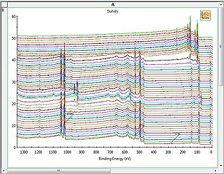
 2D Chart view
 -
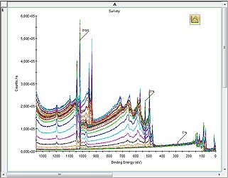
 Stacked Chart view
 -
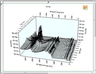 3D Chart view
 -
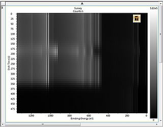 Image view


Automatic peak identification of survey spectra
In the top are several buttons in the 'Analysis' toolbar. Click the leftmost one called Automatic Survey ID and a automated peak identification routine will commence. The result is shown below:

Several things are worth noting:
- A peak table pops up above the spectrum. It contains information (which elements, fitted atomic percentages etc.) obtained in the automatic fitting routine. One can still scroll through the levels (if more levels in a depth profile are available) but the elements fitted will not change.
- Only a fraction of the peaks in the spectrum have labels. The reason is that only the peaks from the peak table have a label - the remaining peaks in the spectrum are NOT unidentified elements but peaks (core levels or Auger transitions) of the elements already identified ni the peak table.
There is two ways of zooming into the spectra:
- Press and hold SHIFT while dragging a square around the area of interest.
- Click the +magnifying glass and a drag a square.
Likewise, to cancel a zoom
- Press 'r' to reset the zoom.
- Click the Xmagnifying glass to cancel zoom.

From here the data may be exported to Excel or Word by using the options on the 'W Reporting' tab next to the 'Display Modes' in the upper right corner of the GUI.
Click here to continue the analysis.