Specific Process Knowledge/Characterization/XPS/Processing/Basics/2highres
Selecting high resolution spectra for peak fitting
The analysis of the data from here is continued. Open a new data grid and drag the four sets of spectra into each quadrant as seen below.

Scroll up or down through the levels of one spectrum by using the scroll button (either etch level or etch time). If several spectra are selected simultaneously by pressing SHIFT or CTRL while clicking on the spectra in the four quadrant view, you watch the evolution of the spectra together.
To analyze a single spectrum, select and maximize it. Before adding peaks to the spectrum, it is a good idea consider what you know about the sample. Here, we know that the sample has ALD deposited layers of ZnO and CuZn on top of a silicon substrate. One would therefore expect to see bulk silicon provided we sputter deep enough and oxidized silicon from the native oxide. Therefore, scroll to a level where, preferably, both the oxidized Si2p and the bulk silicon Si2p are visible. In this case, it is level 35.
-
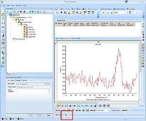 Level 34: The oxide peak is barely visible.
 -
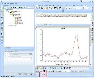 Level 35: Both the oxide and the bulk peak are visible and clearly separated.
 -
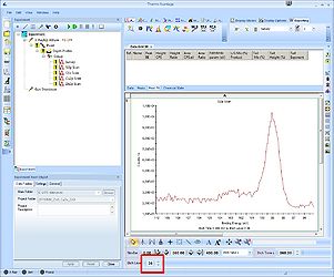 Level 36: The separation between the peaks is less visible.


Click the 'Peak Fit' button in the top to enable peak fitting on all levels.

Peak fitting
A window labelled 'Peak Fitting' with a suggestion to a peak (see red square) will pop up. Usually the peak is correctly identified, in this case it's a Si2p doublet. The window has two tabs - first we will set up the 'Add Fitted Peak'.

In the spectrum the location and width of the peak are shown with bars (see blue square) - you can modify the location and the width using the mouse. Here we start out with the bulk peak as shown. Once this peak is fixed we will add the Si2p oxide peak.
The green square holds the information on how to correct for the background. In this case we will use the 'Shirley' background with default settings.
Click 'Add Doublet' once and the Si2p doublet will be added.

A table with peak fitting parameters emerge above the spectrum. The Si2p spin-orbit couple is labelled Scan A. The details of the fitting is not discussed yet.
Also, in the upper part of the spectrum the residuals of the fitting are shown.
To add the oxide peak, move the centre bar onto the oxide peak (this is why it is a good idea to have both peaks in the same spectrum) - in this case at around 102.8 eV binding energy.
Cick 'Add Doublet' to add the oxide peak.

Swithc to the other tab labelled 'Fit Peaks' in the 'Peak Fitting' window. Here, a button labelled 'Fit All Levels' will apply the fitting parameters to all levels (supposing several levels are available). Upon completion of the fitting routine, press 'Accept' and 'Ok'.
Verify correctness of fitting routine
What looks good in one spectrum, however, may not necessarily look good in another. Click the 'Open Experiment/Instrument And Properties View' button to remove the properties view and enlarge the 'Peak Fit' table. Now scroll through the different levels and notice how the peaks dance back and forth in the spectrum.

In the spectrum above (Level 0), the two doublets slided apart. With only background signal to adjust to, the fitting routine found a minimum with peaks in each end of the spectrum. Below, with a large and pure bulk Si2p spectrum at level 48, the doublets lie on top of each other.

This fitting is clearly wrong and we need to apply some constraints on some of the parameters. Scroll back to a level where all peaks are visible, in this case level 35, see image above.
The Peak Fit table is shown below. The two Si2p spin-orbit doublets (the bulk and the oxide) are referred to as Scan A and B. The various fitting parameters for each of the four peaks are shown in the table along with their constraints. Under each peak is a row with the constraints (in bold) that are to be applied to the parameters.

Going through some of the constraints